Bad Statistics: My Mistake

I was watching this video today and one comment the speaker made was that men's incomes have not increased but women's incomes have. I thought this was interesting and decided to look into it.

However while I was thinking about it I realized that in my last wage analysis I was using 1986 vs. 2006, which wasn't a great idea.

Here's why. What's the difference between this graph:

And this one:

Although these graphs look nothing alike, when you only have two data points you can't actually tell which of the two graphs created this.

That's the issue with my last analysis. We have these weird things in the economy called "business cycles" which you may have heard of, where the economy is doing "well" or "poorly". Unfortunately these cycles could screw up the analysis that I did before since it could be possible that wages haven't gone up at all in a general sense, it could have just been the case that in different economic states in 1986 and 2006 rather than that wages have actually gone up. In 2006 for example, the Canadian economy was doing very well due to high commodity prices, where 1986 wasn't a very big boom period.

This is an example of a very basic statistical problem: model misspecification. In many cases when you're doing statistics you have some sort of model that you are trying to fit the data to. If the model you propose is correct then cool, but if it is incorrect you might not know. Many statistical procedures such as least-squares regression will still work when you give a bad model, but will give meaningless results. Unfortunately it might be the case that the results look reasonable, but are still completely incorrect - this is the most dangerous case, since without further analysis there is no real indication that your results are wrong. Fortunately there are tests like the RESET test that can test for this kind of thing, however you have to know about them in order to actually use them (obviously). They also aren't foolproof - on one hand they will tell you that you do have misspecification, on the other hand they will tell you that you might not have it. As with most things in statistics, you don't get a crisp yes/no answer.

The moral here is that even if you have a representative sample and you have good intentions (ie. not screwing with the results so things look the way you want them to) you can still get bad results by applying the wrong procedures.

Back to the original question: how have wages changed over the years with respect to men and women? Keeping in mind all the stuff that I just said, here are the results:

Median income (2010 dollars)
	1986	2006
Men	37472 (106)	38442 (182)
Women	19331 (72)	25628 (87)

The numbers in brackets are the standard errors, this is how statistics are reported in real papers. If you ever read a paper that reports statistics with comparisons, you should see if they show these numbers. If not, you can't really be too sure about the comparisons - a good example is a survey on game piracy that I critiqued a while back.

So women's wages have gone up a fair bit, while men's wages have not - consistent with the claim in the video. Whether this is a general trend or some blip due to the time periods chosen we can't say with the data here. I can probably find data if I dig around a bit if people are curious.

Empirical SoEn is Hard: Unobservability

One thing that I find interesting is attempting to apply some of the methods of econometrics and labour economics to measure productivity within software development. At the moment it seems like many of us (myself included) base our opinions of "what works" from our own perspectives and from anecdotal examples (which I've said before doesn't really count as evidence for something) - although this here is an anecdote which may or may not be true.
It would be nice if we could come up with some good analysis techniques to give real support to our claims of what works and what doesn't, and better yet when something works and when it doesn't.

It turns out though that tackling the problem of measuring productivity within software development is quite hard. There are all sorts of problems that can arise here that make analyzing data and testing hypotheses rather difficult. This article will be the first in a series talking about some of the problems that I've though of, and I'd be more than happy to hear about what you guys might think about these issues.

The first problem is that of unobservability (also known as latent variables), which is where you are unable to measure a certain variable because you can't really see the variable directly the same way we can with observed variables. An example of this is ability: it is common knowledge (I think) that there is varying degrees of ability when it comes to developing software. But can we give somebody a stamp saying, "this person has productivity X?" Sure, we can use some indirect measures like lines of code produced per hour or bugs closed per day or some junk like that, but these are simply proxy measures that are the result of ability, not ability itself. Compare this with observed variables like years of experience, or language/methodology used, or team size: we can directly give a value for these variables with some specified unit, so therefore they are observed.

These types of variables are problematic because it is difficult to hold them fixed. Since we can't observe them, we often end up with some omitted variable bias as these variables are often correlated with our other observable variables. This happens when we see an increase in productivity and think it is due to one of our observed variables, when it is actually caused by an unobserved variable that is also influencing an observed variable.

I've thought of a few unobserved variables in software development, feel free to add any more that you think of:
1) Ability (the obvious one). I've already talked about this one to death, so I won't go into much more detail here.
2) Team Chemistry. You can throw a bunch of people into a room together, who individually are extremely good at what they do, but doesn't mean they'll get a lot done - if they all sit there bickering over testing frameworks or variable names or other things like that, they're not going to get a lot done. Likewise you can put a group of people together who may not be super geniuses, but if they work well together you still end up getting some good results. This is an important factor in a team's productivity, and you can't really stamp a number on it.
3) Productivity itself. All this time I've been talking about measuring the effects of various factors on productivity, but we don't actually have a way to directly measure productivity. You can see the indirect effects of the productivity: milestones get reached sooner, bugs get fixed faster, less bugs get introduced in the first place, etc. etc. But we don't have a measure to say something like, "the combination of development methodology X with N programmers of E experience and ... gives us P units of productivity."

I thought about putting the complexity of the project in, however I'm not sure if that affects actual productivity. It can affect some metrics used to measure productivity, but if you view productivity as how much someone is getting done per unit time, then I don't think complexity makes a difference in the same way that say for example, having two monitors does. Maybe I'm also on crack and need to go to bed soon, so this point is up for debate.

All these unobserved factors in software development make things rather difficult to do real quantitative analysis. One possible solution is using experiments to analyze various factors, however those come with their own set of issues that I will discuss in future posts.

Values of Different Degrees

As I said in my last post, I would put up some details about how much various types of degrees were worth, according to Canadian census data - as I said in the last post, this type of data should be fairly similar across countries that have similar economies as Canada, like the US, UK, or Australia. I'll make my code available so that if you want to test against your own country, you shouldn't have too much trouble.

Let's take a look at what we have. Here is a ranking of the types of degrees based on a 95% confidence interval of median 2006 incomes (all the values are inflation-adjusted to 2010 Canadian dollars):

1) Engineering: $54.4k - $58.4k
2) Commerce: $51.1k - $55.2k
3) Sciences: $49.8k - $54.3k
4) Education: $47.4k - $48.6k
Median income for university graduates: $45.3k - $47.5k
5) Social Sciences: $43.2k - $46.2k
6) Health/Food Sciences: $38.5k - $42.3k
7) Humanities: $35.0k - $37.4k
8) Fine Arts: $24.5k - $28.4k
Median income for non-university gradates: $25.5k - $25.8k

So it looks like engineers are on top, although their confidence interval has some overlap with commerce graduates which means that if we want to be 95% sure we are right, we can't say that engineers make more than commerce grads. If we reduce our confidence in our results, the data says that once you get down to about 80% confidence you can say that engineers make more than commerce grads. In other words, given our data here, there's a roughly 80% chance that engineers make more.

In the last post I also looked at the data from 1986. Let's see how the rankings change over time:

1) Engineering: $67.4k - $70.8k
2) Sciences: $53.1k - $56.4
3) Commerce: $51.7k - $54.7k
4) Education: $49.0k - $51.0k
Median income for university graduates: $47.9k - $48.9k
5) Social Sciences: $42.7k - $44.8k
6) Humanities: $38.6k - $40.7k
7) Health/Food Sciences: $35.3k - $38.7k
8) Fine Arts: $23.9k - $28.6k
Median income for non-university graduates: $23.0k - $23.2k

The most striking difference between these results and the ones from 2006 is the drop in wages for engineers. They used to be, by far, the most well-paid university degrees, whereas now they are only slightly higher than commerce degrees (which haven't changed all that much). This is somewhat disappointing for up-and-coming engineers (well, necessarily)!

The rest of the degrees haven't changed too much. A couple of them have statistically significant changes (such as education), but for the rest we can't really distinguish any change here from statistical noise - at least not at a 95% confidence level, if we accept a higher probability of being wrong then we can say things have changed.

This analysis here focuses on the median. Why do I do that? Why not use the average/mean? This is because incomes are something that are very skewed, meaning that that the average will be influenced a lot by the outliers that make tons of cash, making it look like a certain degree may be worth a lot when in fact most of the people with that degree are making a lot less than the average. The difference is most pronounced with commerce degrees: in 2006 the average income for a commerce degree holder is around $78k, which is the highest average for all the degree types. However the median is roughly $53k, showing that there is a massive amount of skewness in the distribution of commerce grads: those MBAs that are making big 6-figure salaries are pulling up the average. To get a feel for how most people with a certain degree are doing it is better to look at the median, which is much less likely to be affected by huge outliers than the mean is.

Again I'll repeat that these are correlations, not causations. In fact since the variance of the incomes for all of the degree types have increased dramatically, that could indicate that your degree is less important in determining your salary today than it was 25 years ago. In order to isolate the actual effect of the degree on wage you'd have to have a more sophisticated model that takes into account all sorts of other relevant factors like age, experience, ability, etc.

As always, the code is available here and the results of running the code are here.

Wages Over The Years

I recently read this article which makes a claim that real average wages (aka inflation-adjusted wages) have fallen over the years and supposedly "continue to fall." I looked at this and thought the idea was preposterous, so I rolled up my sleeves and did some real data analysis. Since I've been talking about statistics, I figured some of you might be interested in this knowledge.

tl;dr: Wages overall have actually increased, but not for university grads. University grads still make more than non-university grads. Income inequality has increased a lot, especially among university grads.

First off, my sources. I grabbed the data from the 1986 and 2006 Canadian Censuses (Censi?). Unfortunately I can't share this data with you since I am not legally allowed to distribute it, but if you have access to a university you should be able to dig it up somehow. This data is probably some of the best you can get, since it is much less likely to have selection biases compared to other surveys - people are legally required to fill this data out.
Second source was the Consumer Price Index (CPI) which can be used as a measure of inflation. That's how I adjust the raw figures in the census data for inflation. Statistics Canada is kind enough to list these figures here. All dollar values in this post will be inflation-adjusted to 2010 Canadian dollars.

Now I know that many readers here are not Canadian, however these results should be similar for countries with a similar economy to Canada like the US, the UK, or Australia. For those of you so inclined you can probably find the same data for your respective country to do the same analysis.

Let's get started. How would you go about figuring this stuff out? Well, you need the data. Once you get that, it's pretty straight-forward. I did my analysis using the following steps:
1) Filter the data. I want to look at people who are at least 15 years old, and have a regular old job. This excludes self-employment. This isn't a huge deal, just keep in mind that the averages here are for employed people.
2) Adjust wages for inflation. This is done by dividing by the CPI for the year of the data (1986 or 2006) and multiplying by the CPI for 2010.
3) Construct a confidence interval for the average wage. This lets us see if the wages between the two periods are actually statistically different. The formula for a 95% confidence interval in R-pseudocode is:

mean(wages) ± 1.96 * sd(wages) / sqrt(length(wages))

The 1.96 is the critical value of the normal distribution (sample averages follow a normal distribution) for a 95% confidence interval.

What are the results? Here's the R output:

[1] "Average wages for all employed individuals:"
[1] "Confidence for 1986: 30221.611097 to 30436.550551"
[1] "Confidence for 2006: 38479.736828 to 38790.160974"
[1] "Standard Deviation for 1986: 27382.937843"
[1] "Standard Deviation for 2006: 52381.845010"
[1] "Median Confidence for 1986: 25083.328237 to 25325.457532"
[1] "Median Confidence for 2006: 29704.694341 to 30054.387142"

What are we looking at here? Well, the average wage in 1986 was roughly $30k/year, where the average wage in 2006 was roughly $38.5k/year. Looks like wages in general are not falling.
The median is a better measure here though, since medians are a bit more robust to outliers (aka those few people who make hundreds of thousands of dollars a year). As we can see, the shift in the median is not quite as big as the shift in the mean, meaning that while the wages have gone up, they haven't gone up quite as much as the mean might indicate.
What does all this tell us? Well it is difficult to say for certain, but it would appear that in 2006 people are in fact making more money (as shown by the higher median), but there are also more people making giant salaries than before which will skew the average. Given the big jump in the standard deviation, we can see that there is an increase in income inequality.

Now, here's the real interesting part. I decided to run this again, but with one more twist: I filtered for people who have a bachelor's degree or higher. Let's see the results:

[1] "Average wages for bachelor's degree or higher:"
[1] "Confidence for 1986: 49543.651801 to 50383.047856"
[1] "Confidence for 2006: 59994.274103 to 61070.608811"
[1] "Standard Deviation for 1986: 37181.295254"
[1] "Standard Deviation for 2006: 82837.561885"
[1] "Median Confidence for 1986: 47938.828738 to 48884.408393"
[1] "Median Confidence for 2006: 46310.094270 to 47522.585319"

The average and the median wages here are much higher in both periods than for the entire group. This gives us a pretty good indication that university graduates make more money than non-university graduates.
However, it would appear that while the average university graduate makes far more in 2006 than they did in 1986, this result is misleading. When we use the median we can see that university salaries have actually gone down slightly over this time period. One conclusion that we can guess from this data here is that there are some university graduates in 2006 that are making huge salaries, while the bulk of the university grads aren't doing quite as well.

So there we have it, some statistical data. While the interpretations of the data and the methods for analysis here are up for debate, the numbers calculated are not. They're taken directly from census data, which is pretty darn good data (unfortunately it might not be quite as good for 2011, since the Conservatives have scrapped the long-form census and I'm not sure if this data will be on the short-form one).

Keep in mind that these are purely correlations, not causations. This data is not saying, "if you get a university degree then you will make more money." This data is saying, "people who currently have university degrees make more money on average."
It is also looking at the aggregate. I'm sure most of you can come up with examples of non-university graduates who are making good salaries, and of university graduates who are not making great salaries. These people are the exceptions, not the rule.

One thing that I could do in a later analysis is split the groups up into the different types of degrees. Both these censuses provide the level of education the people get (Bachelor's, Master's, etc.) and the discipline (sciences, engineering, arts, etc.). However this post is getting long enough, so that can wait for another day.

For the code, it is written using R and is available here as a gist on Github. Feel free to fiddle with it if you feel like it. You'll notice I generate some histograms of the data, however I found that they don't really reveal much info so I didn't include them here.

Software Metrics and Instrumental Variables

I recently read this article about how software metrics are mostly useless and tend to cause more problems than they solve. This reminded me of a topic in stats which apparently has some application in software development.

The use of software metrics is an example of a statistical technique called instrumental variables. Often when you want to understand some phenomenon or relationship, you run into problems because many factors are unobservable. This means that they are not concrete things that you can stamp a number on to get a clear measurement of the factor. One example that constantly crops up in economics and software development is ability. A person's ability can have extremely strong effects on other factors such as productivity, wage, etc. However, you can't really come up with a solid measurement for a person's ability: suppose some programmer you know has an ability of 10. What's that mean?
Compare that to a metric like lines of code per hour. A measurement of 10 has a very clear and concrete meaning: given the changes that they made in the hour, the code they have produced contains 10 newlines.

This is where instrumental variables come in. An instrument is an observable variable that you use in place of the unobservable variable that satisfies two characteristics: it has to be correlated with the variable that it is standing in for, and it can't be correlated with random errors or other omitted factors. The power of the instrument is based on the strength of the correlation between the instrument and the unobserved variable. This is why people use things like lines of code per hour, years of experience, etc. etc. for attempting to measure the productivity of a programmer.

Unfortunately there are a number of shortcomings with the instrumental variables method. The biggest issue is finding a good instrument. We know the criteria required for a good instrumental variable (there's all sorts of math proofs that you can look up if you like), however that doesn't mean that there are any instruments that satisfy it. On top of that when dealing with people who know the metric you're using, they can perhaps attempt to cater to the metric - thus introducing a correlation between the instrument and other omitted variables like their ability to cater to metrics.

In short, the problem is not entirely with the method, but more with finding good instruments. Unfortunately if you can't find a good instrument, you'll have to resort to a different method. According to a stats professor of mine, one method for dealing with unobservable factors is to use what's called a mixture model. It supposedly works, however the procedure appears to be much more complicated and can be less precise than having a good instrument. I'm still working on figuring out how to do this sort of thing, perhaps I'll talk a bit more about it another day.

Biasedness and Consistency

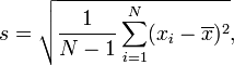
I remember back in those days when I was taking my first statistics class when this formula appeared (hotlinked from Wikipedia):

I thought to myself, "self, holy crap! That's nasty!" (there are actually a lot of nastier formulae, but I was young in my academic career and hadn't seen too many of them yet). At the time all I did was just memorize the formula and promptly forgot it after I had finished the course.

After I started taking economics and I had to take a lot more statistics, I started to wonder why this equation is the way it is. It turns out to be a bit interesting, and you can learn a bit about statistics when you answer this question.

The part that I thought was the weirdest is that when you take the standard deviation of the population you divide by n, however when you take it from a sample, you use n - 1. Why did the do this?

Let's go on an aside for a bit. When we are using a sample, these statistics that we are generating (the sample mean and the variance) are estimators of the actual parameters, based on the sample that we have taken. These two estimators are random variables, which means it is highly unlikely that they will be the same as the actual parameters. This is not a bad thing, however we would like to have some measures of "goodness" of the estimators that we have.

One measure of "goodness" is called unbiasedness. Intuitively we all know what a bias is, it is something that sorta skews the estimate away from the actual value that we are estimating. Formally you would call the estimator unbiased if:

E(estimator) = parameter

The E function there is the expected value of the random variable, which is essentially an average value that the random variable comes out to. If on average the estimator is not coming out to be our parameter, then we have some kind of bias going on.
Given the above definition, our variance estimator would be unbiased if:

E(s2) = σ2

It turns out that if you divide by n for the sample variance you end up with:

E(s2) = &sigma2 * (n - 1) / n

This is always smaller than the variance, so our estimate is biased downwards. Thus we must correct the bias by dividing by n - 1 instead of n.

So that's why you divide by n - 1 and not n. While that's almost enough statistics for you for one day, there is one last tidbit of information that can be taught here. If you look at the formula for the expected value of the biased estimator, you'll notice that the bias will shrink as n gets large. In fact in the limit, the bias will go to zero and you will have an unbiased estimator. The name for this type of estimator is a consistent estimator. While they are not as good as unbiased estimators (note that all unbiased estimators are consistent), it is often the case that you might want to use a biased yet consistent estimator instead of an unbiased one if perhaps there is something wrong with the variance of the unbiased estimator. Eventually in one of my statistics posts I will talk about some problems with real-world data that might cause this sort of thing to happen.

Statistical vs. Practical Significance

A lot of my statistics posts have talked about this thing called "statistical significance". To repeat for the millionth time (it's that important), when you say something is statistical significant it means that it is not likely that it occurred just by some random fluke.

Statistical significance isn't the only type of significance you should care about. Another type that is important is practical significance. Something is practically significant when you actually care about the results for some practical reason like cost, effort, etc.

Let's look at an example. Suppose we have some code and we want to make some changes. After we make our changes, we want to compare the new version against the old one for something, like performance, memory usage, etc. In this example we'll look at performance. The old version took on average 50ms to run and the new version 10ms. I'll omit the standard errors, just assume that if I say the result is statistically significant then the standard errors are small. Here are our four cases of significance:

	Practical	Not Practical
Statistical	In this one suppose our change is switching data structures in a render loop of a video game. The improvement of 40ms is huge, so it has a high practical significance.	Suppose here the difference is a change in the processing time of a PHP script on a website. The result is 40ms faster, but does it really matter?
Not Statistical	Suppose we're back in the video game render loop. If there is no statistical difference between 50 and 10ms, then we have a huge problem - our standard errors are huge. It means some frames will render quickly while others will render slowly. This is a practically significant result.	This could be a change to a cron job that runs every night at midnight. You make a small tweak that doesn't really have an effect on performance. There is no need to speed things up, so it doesn't actually matter whether the result is statistically significant or not (assuming that the standard errors are still reasonable, ie. not more than several hours).

Hopefully these examples illustrate the difference between statistical and practical significance. In short, statistical significance is mathematical - it comes from the data and from your confidence (how confident you want to be in your results). Practical significance is more subjective and is based on other factors like cost, requirements, etc. Neither one implies the other, there are situations when one or the other may exist but not both.

The Plural of Anecdote is Not Data

One common logical fallacy that people use in arguing (especially online) is using anecdotal evidence as actual evidence. This means that they find some example of something that corresponds with their argument, and use that example as evidence to support their argument.

You might think at first, "what's so bad about that? They're using evidence to support their argument, isn't that what you're supposed to do?" Yes, I suppose this type of argument is better than just pulling something out of your ass with absolutely no evidence behind it (which is probably just as common online as anecdotal evidence). However, that doesn't mean it is good. The issue is that for pretty much any side of an argument you can find an example that supports that argument. A common one that is loved by the Canadian Pirate Party is, "so-and-so artist says that he/she likes piracy because it boosts concert sales, therefore piracy is good." This could be a legitimate argument, and economically it is possible - reduction in the price of a good (the music) increases demand for a complement good (the concerts), but without detailed statistics the effect is ambiguous to the musician's overall welfare. The problem is that one example alone does not provide a justification for the argument. Instead you would need a lot of data from a good sample to verify the actual effect.

From a more formal standpoint, the root of the problem is a sampling bias. You are taking a potentially non-representative subset of the population and claiming that it is representative. There is no guarantee that this particular anecdote is representative, so any conclusion you derive from the anecdote about the population isn't really valid. In the example in the last paragraph, they're using a subset of a subset of the population (a few musicians do not represent all artists).

This isn't to say anecdotes are all bad. You can derive useful insights about larger phenomena by analyzing anecdotes, for example asking "why do certain artists like piracy" can lead you to the basic economic analysis that I mentioned earlier. However it ends at the insight, if you want to derive a conclusion about the population with this insight, you have to resort to more advanced statistical methods.

Piracy Boosts Game Sales? Yeah right...

Some pirates in the Canadian Pirate Party are getting all excited about a certain paper, part of which says that file-sharers tend to buy more games more often than non-file-sharers.

First off, let's address some problems with the paper. The paper says that 61% of file-sharers have bought games in the last 12 months, vs. 57% of non-file-sharers. They say that this is evidence that file-sharers buy games more often. I say that there isn't enough information here to say who buys games more often. They don't specify any type of variance in the paper, so you can't actually say if the difference between these two figures is actually significant (this is an example of a difference of means).
The other numbers are 4.2 vs. 2.7, which represents the average number of games bought over the last year by file-sharers and non-file-sharers respectively. Again there is no mention of a variance measure, so you can't really take this difference seriously.

Next, they claim that only 53% of their sample answered questions about games. If their sample was random before, it's probably not anymore! This is an example of a self-selection bias. It could be that all the people who pirate games and never buy them chose not to answer the question, or it could be that people who always buy them and never pirate also chose not to answer (this one I think is a bit more unlikely, but not impossible). Basically you no longer have a guarantee that the sample that actually answered the questions about games is a random sample.

The next problem is with addressing the interpretation of the paper. Some people seem to think that this result shows that piracy causes more sales, and overall is a good thing for the gaming industry. This is a definite possibility, and the paper addresses this and claims it is due to something called the sampling effect - an example of this effect is trying a sample at Costco, you trying the good might increase your demand for it. I completely agree with this, it's entirely true that piracy can increase the demand for a game because they get a chance to try the game before they buy it - I've personally experienced this, I pirated Half-Life 2 and Oblivion and then later bought them because they are awesome games.
However the effect can go the opposite way. A lot of games are only fun the first time you play them. What might happen is that the person will pirate the game, play it through, and then never want to play it again. They may have loved the game, but don't really want to shell out the cash to buy it and not play it anymore. An example for me was Spore - it was kinda fun the first time around, but after I realized that the game wasn't really interesting for very long I had no incentive to buy it (let's ignore DRM-related issues for the moment too). In this case I might also say piracy would be a good thing, since it gives game creators an incentive to make games that don't suck.

It is also possible that there is no causal effect at all between these two. It could be that those hardcore gamers out there who buy a lot of games also pirate a lot of games; while the casual gamer who maybe buys a game once or twice a year has no idea that he can pirate a game or has no desire to "break the law" for something he doesn't really care about.

Anyway none of these points prove the paper wrong, however they show that you shouldn't really trust the results. If I saw several more studies come up that actually show the data that points to the same result then I might be more convinced, but for now I'm very skeptical of whether or not this paper is valid.

Computing P-values

A commenter named Blues asked me a question on my post about differences of means:

... could you explain how to do the math without R? ie, if I wanted to do the calculations on paper, or write this in javascript, what are the formulae I'd use, and what's the logic behind them?

This question is about calculating the p-value for a statistic.

Unfortunately this is not that simple a problem. If you're using the standard normal distribution, the equation looks something like this:

f(x) = 1/sqrt(2 * pi) * exp(-x*x/2)

It's not a terrible formula, however the main problem is that the p-value is an area under this curve, and this function has no anti-derivative. This means that in order to calculate the integral, you need to use numerical methods instead of the traditional way of solving the integral.

Single-variable integrals for nice continuous functions like this are not very difficult at all using numerical methods. It amounts to just adding up the area of boxes. The smaller the width of your boxes, the more precise you will be.

In our case, we're trying to calculate a p-value. The first thing you need to decide is if you're doing a one-tailed or a two-tailed test. In a two-tailed test, you're saying in your null hypothesis that the thing you are trying to test is equal to some certain value, call it c. Therefore if your statistic is either much lower or much higher than c, you reject the null hypothesis. In a one-tailed test, you're using an inequality in your null hypothesis. You'd say something like, "the value I'm trying to estimate is less-than or equal to c." Therefore you'd only reject the null hypothesis if the test statistic was much higher than c.

In the end, there isn't a huge difference in the math. You compute some value, and in a two-tailed test you'll multiply this value by 2.

So what is the code to do this? Well we need to first define our problem. What we're doing is the more general concept of integration of a function between two values. The Javascript version (I'll use Javascript because that was the language asked in the comment) looks like this:

function integrate(a, b, f){
  // what we are trying to do is find the area under f in between a and b
  // assume that b > a
  var dx = (b - a) / NUM_BOXES; // NUM_BOXES is some large constant
  var x = a;
  var sum = 0;

  while (x < b){
    // add on the size of the box
    sum += dx * f(x);
    x += dx;
  }
  return sum;
}

This algorithm is pretty good, but in the case of a decreasing function it will always over-estimate the area, and for an increasing function it will always under-estimate the area. You can get a better estimate by using a mid-point:

sum += dx * f(x + dx / 2);

It's pretty obvious that the larger NUM_BOXES is, the more precise your result will be. However it will come at a cost, the number of times the loop is executed depends on the value of NUM_BOXES. For our p-value, what we want to do is calculate the area under the normal distribution from the absolute value of the calculated statistic (from now on I'll call this value z) to positive infinity. Unfortunately since we can't go to positive infinity, we'll have to stick to some high number. Since the normal distribution drops very quickly, once you're past a value like 5 you have a pretty decent approximation. If you want more precision, go higher. All that said, you'd calculate your p-value like this:

pvalue = integrate(Math.abs(z), 5,
  function(x){
    return 1 / Math.sqrt(2 * Math.PI) * Math.exp(-x * x / 2);
  });

If it is a two-tailed test, just multiply this value by 2. So this is for the normal distribution, but it wouldn't be too hard to figure it out for more advanced distributions like Χ² or t. You just need to plug in the correct formula for each distribution and then off you go.

A Little Intro to Time Series

One thing you might have never heard about in an introductory statistics class is this thing called time series. It's a pretty simple idea, it's just a collection of measurements of a variable over time. Lots of economic variables are time series variables: GDP, nominal prices/wages, stock markets, etc. Also, lots of variables within the computer world are time series: CPU clock speeds, hard drive capacities, number of programmers in the marketplace, etc.

These types of variables are interesting because they have certain properties. The main one is that they are highly correlated with one another when the observations are close together - for example, the average clock speed for a CPU sold in a certain year is going to be pretty correlated with the average clock speed for a CPU sold in the year after.
Compare this to something that isn't a time series, like the time it takes you to run a piece of code. Comparing the first test to the second test isn't really any different than comparing the first test to the hundredth test. However comparing CPU speeds between say 2001 and 2000 is a lot different than comparing CPU speeds between 2001 and 1970.

It turns out that this really messes up your results when you want to use linear regression to analyze relationships. I went off to Statistics Canada to get some data for an example (I can't publish the data here, since it isn't mine and it isn't open - you can change this by helping out with open data movement). I took two variables and checked out their relationship to one another over time, from 1980 to 2008. Using my trusty StatsAn tool, I was able to fit a line between two variables with a very strong level of statistical significance. I know it was strong because the t-statistic for this variable was 18.8 - the probability of getting this t-statistic with this sample size if there is no relationship is 0 if you round off at 6 decimal places. Yikes! What were the variables that could have had such a strong correlation?

The dependent variable in this example is the population of Canada, and the independent variable is the logarithm of the capacity of hard drives in gigabytes. According to my analysis, the capacity of hard drives over the last 30 years has been a very strong driver of the Canadian population growth.

Hmm.

I think something is wrong here.

And in fact, there is something quite wrong here. The thing that is very wrong is that there is an omitted variable bias. However in this case the omitted variable bias is a rather unique variable - time. Consider the following two models. The first one I did is this:

population_of_Canada = β0 + β1ln(hard_drive_capacity)
population_of_Canada = β0 + β1ln(hard_drive_capacity) + β2year

The added variable here is the year of the measurement. When you add year to the mix, the t-statistic for β₁ goes from 18.8 to 0.65. With this sample size the probability of getting a t-statistic like this is over 50% when the relationship between hard-drive capacity and the Canadian population is non-existent (assuming that our model is correct). That's a pretty high probability! So basically the portion of Canadian growth that was actually due to time was being attributed to the increase in hard drive capacities over the years - thus giving us a strong positive link between the two.

Anyway the moral of this story is a fairly obvious fact: it is easy to find a "relationship" between two variables over time when you're not compensating for the fact that those variables are changing over time.

Book Review: How to Lie with Statistics

I've recently just finished reading a book called "How To Lie With Statistics" by Darrell Huff. The name says it all, it is a book that talks about a lot of the basic misconceptions that people have about statistics, and how some content writers will abuse those misconceptions (knowingly or unknowingly) in order to get a message across.

It was published quite some time ago (1954) but it is still quite relevant. While statistics has advanced a fair amount in that time (well I'm not sure about statistics itself, I assume it has, I know that econometrics has) the way people perceive basic statistics hasn't changed all that much.

So anyway, if you have been reading my statistics posts and like them, I recommend you check this book out. It's not quite as technical as the stuff I've been posting - which may or may not be a good thing depending on how you look at it - so it is a nice and easy read while you're on the bus or metro/subway. Oh, and there are lots of pictures, which are sometimes kinda funny and usually quite helpful.

Testing Random Numbers

After reading Cryptonomicon where they spoke a lot about random numbers, I was a bit curious about how that kind of thing all works. I remember when I took a course on cryptography we very briefly scanned over the topic, it had to do with discrete modular logarithms or something like that (it was a few years ago and my memory is a bit foggy), and more recently I was interested into looking into this a bit further. So I grabbed a copy of The Art of Computer Programming, Volume 2 by Donald Knuth from Concordia's library which covers random number generation in a fair amount of detail. It's quite interesting and I encourage you to grab a copy for yourself and check it out. The book is a bit dated and heavy in the math (which I know some programmers hate) but it is still a good learning experience.

While I was reading Knuth talks a bit about how to test to see if a sequence generated by a random number generator is actually random. I decided to stop reading there to see if I could think of a way to figure out this test myself. Here's my guess: if the correlation between the nth number generated and the (n + 1)th is zero for all n, then the sequence is random. Of course this is probably not an amazing test for randomness, but it is still fun to play around with.

How would you go about testing this? Well, I've been writing posts on statistics, so why not take a statistical approach? I'll generate a sequence of random numbers, and then do a regression on this equation:

ni = α + ρni - 1 + ε

What does this mean? Basically it measures the effect of a value produced by the random number generator on the next value that is produced. This effect is captured by the variable ρ. If it turns out that ρ is not statistically different from zero, then I can conclude that the sequence is random. The α is the average of the random number generator - for Ruby it is 0.5 since rand gives you a number between 0 and 1, with C the average should be RAND_MAX / 2.

Here's how we go about testing a random number generator. I'll be testing Ruby's built-in rand function. You can use a statistical tool like R to run this regression, however I will be shamelessly advertising my StatsAn project for this post.

First, the data. This code will put 27982 random numbers into a CSV file, which is what StatsAn uses at the moment (I just picked 27982 out of thin air, use whatever you feel like).

File.open("output.csv", "w") do |f|
  f.write("n\n")

  1.upto(27982) do
    f.write("#{rand}\n")
  end
end

You can load this file into StatsAn by clicking "Import File" at the bottom and uploading the file. It will take a sec to upload.

When it's done, you'll see on the left bar under "Datasets" there is an n there. This is the dataset. You can run the regression equation that I mentioned before by clicking the command field at the bottom and running this command:

regress n lag(n)

This spits out a whole bunch of numbers related to this regression (looking at them real quick I realized not all of them are totally correct, but the ones related to this example are). The ones we're interested in are in the big table at the bottom. There is a row named int which is the information about the intercept. The estimate for this is under the Coeff. column, which for me is 0.50159; and the confidence interval at 95% confidence is the Lower 95% and Upper 95% columns, which for me is [0.494806, 0.508382]. Since 0.5 is in this confidence interval, the estimated intercept (aka the α from our equation) is what we would expect.
Next, the coefficient estimate for the lagged value for my sample is 0.001113, which is pretty close to zero. This number reflects the correlation between the two generated random numbers. If we look at the p-value for this number it is 0.852255, which means that if the actual value of ρ is zero, then we have an 85% chance of getting a sample that gives us the estimate that we got. That's a pretty high chance, so we can't say that the actual value of ρ is different from zero. Therefore our estimate of ρ is not statistically different from zero, so we conclude that the generator is random.

Anyway as I said before this probably isn't a perfect test - I stopped reading the book to see if I could figure things out for myself, since that's how programmers roll! There are probably better ways to test the randomness of a random number generator. On top of that, there are probably a number of statistical problems with this that I haven't thought of. However it is a fun little example, and it is an easy way for anybody interested to fiddle around with a statistical tool.

UPDATE: There could indeed be problems with this. If it is the case that the system is actually random then we are fine. The problem is when the system is not random, then our test here might be a fair bit broken. Unfortunately the problems with it are a bit more advanced than anything I've talked about, so I won't go into detail on any but one: suppose the nth element is correlated with the (n + 1)th element, and it is correlated with the (n + 2)th element. Then we have an omitted variable bias here which might mess up our results.

By the way, if you notice any problems with StatsAn, let me know. It is still beta software!

Statistics For Programmers VI: Omitted Variable Bias

This entry is part of a larger series of entries about statistics and an explanation on how to do basic statistics. You can see the first entry here. Again I will say that I am not an expert statistician, so feel free to pick apart this article and help bring it closer to correctness.

In the fourth post in this series, I spoke briefly about the assumptions required for using regression to analyze your data. One of them was about the error term having zero mean conditional on your independent variables - this means that if you hold your independent variables fixed, then the average of your errors should be close to zero.

There are certain situations when this assumption can be violated. One common one that I'll be talking about today (obviously, given the title of the post) is called omitted variable bias. This occurs when you don't include an independent variable that has an effect on the dependent variable, and also is correlated with other independent variables (I believe omitted variables are also called confounding variables). What happens when you use ordinary least squares is that your regression doesn't know that the variation in the omitted variable (let's call it c) is causing changes in the dependent variable (call it y). Assuming that c is correlated with an independent variable x, the regression cannot tell whether the variation in y is being caused by x or by c since you haven't included c in the model. Therefore it will attribute all of that variation to x.

Let's look at an example. Suppose you've been arguing with someone on reddit about agile vs. waterfall and you want to prove which one of these makes programmers more productive (while I don't know if one is actually better or not, let's assume for illustration purposes that one of them is). Now suppose you've read all my previous posts on statistics, and you've taken a course in statistics in university, so you feel fairly confident in your ability to do statistical analysis. You go out and start collecting some data from various companies (suppose they cooperate and give you their data, and that it is reliable). You collect various types of data: how big their team is, the experience of the team members, the language(s) and libraries they're using, and finally whether they are using agile or waterfall. Also suppose you have some reliable way of measuring productivity (this is another one we'll have to assume, since measuring programmer productivity isn't that easy). So you run a regression on all this and it turns out that agile has a significantly larger effect on programmer productivity than waterfall. You post your results on reddit and say, "Ha! The data says so!"

Unfortunately there is a problem here. What you haven't included is the average ability of the programmers at the various companies. It is fairly certain that the average ability of your programmers will impact productivity (of course that will require you to hold constant any synergistic effects between programmers - see, this stuff is hard!). Again for illustration purposes let's pretend that hot-shot programmers like to work in agile environments rather than waterfall environments, so the average ability for programmers will be higher for agile than for waterfall. So we have an omitted variable that is correlated with both the dependent variable (productivity) and the independent variable we are interested in (agile vs. waterfall). This will bias our estimate for the effect of agile vs. waterfall, and the size of the bias typically looks like this:

bias = (effect of average ability on productivity) *
    (correlation between average ability and agile vs. waterfall)

Since these are both assumed to be positive values, the bias will be positive (since I'm assuming ability has a large effect on productivity, this bias will also be large) - the effect of agile will be very much overstated in your analysis.

Of course, you could always decide to lie with your statistics and hope that your target audience doesn't know very much about statistics to properly argue against your results (especially if you include math, they might not even read the analysis!). This is not a very respectable thing to do, but that doesn't stop people from doing it anyway - how many statistics do you see in the newspaper, magazines, blogs etc. that do not include a standard error and confidence interval? or when they say average/mean, do they say which type of average/mean? or do they tell you their sample selection methods? I could go on like this for a while.

Anyway let's assume that you decide to do everything legit and you want to control for programmer ability. The problem with this is how do you give an objective number to each programmer? Sometimes in labour economics worker ability is treated as an unobserved variable, which is a variable for which you cannot get a good quantitative value. So how do you go about measuring this? There are some techniques that have been developed like instrumental variables which can help, but typically you're going to have to make some trade-off between biased results and imprecise results.
In fact, productivity may also be considered an unobserved variable!

On another note, I'd like to get some feedback on these posts. Do people find them helpful, or am I just boring you with what you learned in your stats classes?

« Statistics For Programmers V: Performance Analysis

Statistics For Programmers V: Performance Analysis

This entry is part of a larger series of entries about statistics and an explanation on how to do basic statistics. You can see the first entry here. Again I will say that I am not an expert statistician, so feel free to pick apart this article and help bring it closer to correctness.

In the last post, I covered a little bit of theory on how ordinary least squares works. This is a method of fitting a curve to a set of points so that you can get estimates of how independent variables affect a dependent variable.

In this post, we'll use that technique in a programming-related example. Let's say we have a task of optimizing code. There's a certain section that is too slow, and we need to figure out why that section is slow and fix it up. Normally 99% of the time, the slow part is in our own code, or it might be in code that you can access and change (gotta love the prevalence of open-source these days!). However in our hypothetical scenario here you're working with a library that is not open-source, meaning that there's not really any way for you to look at the code to analyze it properly. So what do you do? Well you could roll up your sleeves, fire up ndisasm (or whatever disassembler you have handy) and take a peek at the assembly code. While this is possible, I probably wouldn't recommend it because you'll be spending so much time digging through everything that you'll be at it all day just trying to figure out what is going on. Then on top of that you'll have to do your performance analysis, which a lot of the time requires some probability anyway.

So, why not attempt to use statistics for it? If you are using a library then chances are the functions/methods you are using have some sort of inputs that they use (the independent variables) and you have some kind of measurable (usually) dependent variable based on those inputs - like the amount of time it takes the function to run, how much memory it uses, etc. What you could do is take various sets of possible input values, and record the dependent variable(s). Then afterward you form a hypothesis and you can test it using ordinary least squares.

What do I mean by form a hypothesis? Well, let's say that you are fairly certain that the algorithm is O(n²). What you could then do is set up your regression equation like this:

T = β0 + β1n + β3n2 + ε

After that you could just run your code over and over with different values of n and collect the corresponding execution times. You can then run the regression on the set of data to get the estimates for the coefficients.

Once you run the regression, most statistical packages will spit out a standard error for each coefficient. This standard error is the estimated standard deviation of the distribution of each coefficient. What does that mean in English? Well, you have an actual value for each coefficient called β, which unfortunately you don't know. If you take a sample of a certain size and assuming all the assumptions are satisfied, it will effectively take a random value from around β that is distributed according to a t-distribution. This distribution has a standard deviation, which again we unfortunately don't know. The standard error is effectively our guess of that standard deviation based on the sample we have.
What does the standard error do? It determines how precise our estimate of β is. If our estimate of β is 100 and our standard error is 0.1, then it's nearly a 100% chance that the actual value of β is between 99 and 101. However if the standard error is 10, then the range that the actual β could be in is much larger. You can get smaller standard errors by increasing your sample size, or by getting a wider range of values for your independent variables.
Note that when some of our assumptions are violated, it can potentially have a huge effect on the standard errors.

We can use the estimates and the standard errors to form hypotheses about the actual values of the coefficients. Suppose our estimate of β is 5, and we want to test to see if the actual value of β is 6. We would then form a hypothesis that β = 6, this is called the null hypothesis. You compute a t-statistic for this null hypothesis using the formula:

est(β) - β) / st.err

If this t-statistic is small (the threshold depends on your sample size and how confident you want to be in your results) then you cannot reject the null hypothesis - this does not mean that the null hypothesis is true, it just means that this sample is not enough evidence to say that it is false. It could be true that β = 5.5, and we could still get a sample like this (depending on the standard error of course). So if the t-statistic is small, we can't say a whole lot about our null hypothesis.
On the other hand if the t-statistic is large, it provides a good amount of evidence that the null hypothesis is wrong. So typically when you test a hypothesis, you let the null hypothesis be something that you want to "prove" wrong (I say "prove" since you can't really have 100% proof in statistics like you can in math).
Most stats packages like R or even Excel will spit out a calculated t-statistic for each coefficient. What this value represents is the t-statistic for the null hypothesis of the coefficient being equal to zero. If that t-statistic is small, we say that the coefficient is not statistically significant - that is, we can't really say that it is any different from zero.

What does all this mean for testing the code? Well it lets us get an idea of how fast the code runs. Suppose we get an estimated equation of:

T = 100 + 30n + 0.5n2

Provided that our standard errors for the coefficients are fairly small, this equation shows us several things. First, it shows that there is a fixed cost to the code. It doesn't really matter the size of the input, we still have 100 there each time you run it. It also shows a fairly small estimate on the n² value. This is useful for comparing this algorithm to another. Suppose you come up with a fancy new algorithm that you figure out runs in O(n) time. This is theoretically better than the O(n²) algorithm, but if the equation looks like this:

T = 2000 + 400n

then the O(n²) algorithm is much better if you're only ever working with small values of n.

So this is a basic introduction on how to use statistics to test performance analysis. Unfortunately, there are still plenty of things that can go wrong. I listed a few assumptions in the last post, if those are incorrect then you can have problems such as biasedness and inefficiency (I'll talk about these more in later posts). Also if your model is misspecified (if perhaps the algorithm is actually O(nlog(n)) instead of O(n²)) then you probably won't get correct results. Fortunately there are tests for this kind of thing that you can do, which I might cover in a later post.

« Statistics For Programmers IV: Ordinary Least Squares | Statistics For Programmers VI: Omitted Variable Bias »

Statistics For Programmers IV: Ordinary Least Squares

This entry is part of a larger series of entries about statistics and an explanation on how to do basic statistics. You can see the first entry here. Again I will say that I am not an expert statistician, so feel free to pick apart this article and help bring it closer to correctness.

In my last post about statistics, I spoke about how to compare two different averages to see if they are statistically different or not. It was a good introduction to using statistics for hypothesis testing since it was fairly simple yet went over some of the fundamental ideas of statistics - that disturbances could result in us coming to wrong conclusions, and we must do our best to try and detect whether or not differences in results come from the disturbances or from what we believe it to be.

This time we'll address something a bit more complex. In many cases we want to analyze a causal relationship between two variables - that is, variation in one variable is causing variation in another variable.

Note that this post is a bit more theory-oriented, the next one will apply the theory to something programming-related.

In econometrics (something that I've been studying a fair bit over the last year or so), a tool used for this type of analysis is the ordinary least squares (OLS) method. This method assumes that the relationship between the variables can be explained by an equation that looks like this:

y = β0 + β1x + ε

Here, y is the dependent variable, x is the independent variable, β₁ is the effect of a one unit change of x on y, β₀ is the intercept term (basically what y is predicted to be when x is zero), and ε is a random error term. This example only uses a single independent variable, but you can have many more. You can also have functions of independent variables in there, so you could put x² if you like. For OLS, the restriction is that the equation is linear in the β terms (called the parameters) - that is, OLS is a linear estimator.

Once we have formulated our model, we can use data to estimate what the β coefficients are. There are plenty of statistical packages out there that will do OLS on a dataset, R is one that is open-source and available for Ubuntu. It's not as user-friendly as other ones that I've used, but it is easier to get your hands on it.

This paragraph talks about how the estimates are computed, feel free to skip it if you don't care. Otherwise if you want to be hardcore and calculate out the coefficients yourself, the math formula is:

est(β) = (X'X)-1X'y

Here est(β) is the estimator of β, which is a column vector of the parameters in your equation (in the example above we had 2 parameters, so it would be a 2x1 vector). The X is a matrix of your independent variables, for the intercept term you just set one of the columns of your matrix to all 1s. Each independent variable occupies one column of your matrix, so the matrix is nxk for n observations and k independent variables (including an intercept term if you have one). X' is the transpose of X.

So now you know how to get take a bunch of data and infer a causal relationship between them, right? Unfortunately it is not entirely that simple. OLS comes with a whole pile of assumptions in order for you to properly analyze the results that come out:

• The expected value of ε conditional on X is zero. That means that if you hold your independent variables fixed and just keep taking observations, the average error will be zero. It is common for this assumption to be violated, and when it is you usually end up with biased results. It is important to understand how it can be violated and what to do when it is. I'll talk about this more in a later post.
• Random sampling - the different observations of a specific variable are not correlated with one another. This can be violated for dynamic systems where the observations are taken over time.
• No perfect multicollinearity - this basically means that no independent variable is a perfect linear combination of other independent variables (for example if x₅ = 2x₂ - 3.14x₇ you would have a perfect linear combination). You're pretty hosed if this is the case, and you'll probably need to end up removing a variable.
• Homoskedasticity - given any value of X, the spread of your error term is constant. When this is violated you can still use OLS, it's just there will be better estimators.
• No autocorrelation - none of the error terms are correlated with the other error terms. With autocorrelation you can still use OLS, but like heteroskedasticity there will be better estimators.
• Normal errors - your errors must be distributed normally with a constant variance. Note that if this is the case then you will have homooskedasticity and no autocorrelation. If this assumption is violated, then you cannot use the hypothesis tests in the same way.

Assuming all the assumptions are satisfied, we can do hypothesis testing on our estimates of the parameters. Fortunately the hypothesis testing here is even easier, since statistical packages usually spit out the p-value for each parameter. What that p-value measures is the probability that if the actual value of the coefficient were zero, then we would have p-value probability of getting the sample that we did. So if the p-value is very small, you can guess that the actual value for the parameter is not zero.

Anyway like I said before, this post was a bit dry and theoretical. I'll get to something more practical next time.

« Statistics For Programmers III: Differences of Means | Statistics For Programmers V: Performance Analysis »

Statistics For Programmers III: Differences of Means

This entry is part of a larger series of entries about statistics and an explanation on how to do basic statistics. You can see the first entry here. Again I will say that I am not an expert statistician, so feel free to pick apart this article and help bring it closer to correctness.

One thing that I've noticed programmers (including myself) do when comparing two versions of code is they run it once for both versions and compare the time it takes. If one is faster, then they conclude that that one is faster and take it.

It is possible that this conclusion is correct, that the faster one is indeed actually faster, however the evidence here is not very good. It is also highly possible that the faster one is only faster because some randomness in the execution time made it seem faster. Take a look at this picture:


Suppose this is the graph of the runtimes of two versions of the same function. The variance is unchanged at 16 (so the standard deviation is 4, which means that the average distance from the mean for a test is 4). The green version of the function has an average runtime that is twice as much as the red version, meaning that it is twice as slow. However it is highly possible that your test for the green function ends up in the left tail and the test for the red function ends up in the right tail, meaning that you'll wrongly conclude that the green version is faster. (Note that another good idea here would be to try and reduce the variance of your function).

In order to get a good idea of which one is actually faster, you need to do some analysis, and for this analysis you need to know the variance of the running time. Unfortunately you cannot get an estimate of the variance with one test (mathematically it results in a divide by zero) so you need to have several tests for both versions in order to create a decent sample. How many tests? That depends on a great many factors, but if we assume that the randomness is a random variable that normally distributed (I'll give a tiny bit of info at the end about what happens if it isn't) then the number of tests depends on what level of confidence you want in your results, and how precise you want your estimates to be. If you want to be 95% sure you are correct instead of 90% sure, you'll either need to accept a lower level of precision or run more tests. On the other hand if you want to be more precise, you'll need to either accept a lower level of confidence in your results, or run more tests.
Finally, the number of tests you'll need depends on the variance of the randomness in your tests. A higher variance will need more tests in order to be more precise.

So let's say we've got some data for our two versions of the code and we want to know which one is faster. Unfortunately it is not as simple as taking the average from one and subtracting the other, since this doesn't take into account the variance of the two distributions.

One way to do this is to compute a new dataset containing the differences between the two distributions. You would do this with the formula (assuming x_t is the tth observation from one version of the code and yt is the tth observation from the second version):

dt = xt - yt

You can then take the average and variance of the ds and make a conclusion. We want to test if the difference is equal to zero, because if it is then we cannot say that there is a difference between these two samples. We do this by taking a t-statistic, which uses the following formula (assuming d is the difference, and n is the size of d):

t = average(d) / sqrt(variance(d) / n)

You then compare this value to the t-distribution with n - 1 degrees of freedom (I'll explain what the degrees of freedom are in a future post) to see what is the probability that we would get this t-statistic assuming that the actual mean of the difference is zero. If this probability is very low, then we can say with a certain level of confidence that we are wrong with our assumption that the mean of the difference is zero. This probability is called the p-value (some people call it the power of the test), and using R you can compute this p-value:

2 * pt( -abs(t), df = n - 1)

This will give you a value between 0 and 1, which is the probability that if the mean of the difference was actually zero, there is a p-value percent probability of us getting a sample that gives us this t-statistic. If this probability is really low, then we can say that it is more likely that our assumption of zero mean is wrong. If the difference is not zero, that means that one of the two versions of our code is faster, which one being the one with a lower average runtime.

You can also do this using confidence intervals. This is where you compute a range, and if zero is in this range then you cannot say that the difference is not zero. With a confidence interval you need some t-critical value for your level of confidence. If you want to be C% confident, you can use the formula in R to get the t-critical value (you divide by 2 because the qt() function in R is for a one-tailed test):

abs(qt((1 - C) / 2, df = n - 1))

You can then create your confidence interval:

lower_bound = average(d) - tcrit * sqrt(variance(d) / n)
upper_bound = average(d) + tcrit * sqrt(variance(d) / n)

If zero is in this interval, then you cannot say that there is a difference between the runtimes of the two functions.

A quick note on normality: we assume here that the randomness in the runtime is normally distributed. If we don't know that it is normal, that means that the "t-statistic" we calculate does not actually follow a t-distribution and the results we get from computing t-statistics and p-values is pretty meaningless. However this problem can be remedied by using a large sample, because as the sample size goes to infinity the distribution of our "t-statistic" converges to the normal distribution, and we can still use the p-value. This also requires a few assumptions, which I will talk about in later posts.

« Statistics For Programmers II: Estimators and Random Variables | Statistics For Programmers IV: Ordinary Least Squares »

Statistics For Programmers II: Estimators and Random Variables

This entry is part of a larger series of entries about statistics and an explanation on how to do basic statistics. You can see the first entry here. Again I will say that I am not an expert statistician, so feel free to pick apart this article and help bring it closer to correctness.

The whole point of statistics is that there are some things that we don't know, and we can't really measure those things - it might be because it costs too much, or we have a lot of measurement error, or it is actually impossible to accurately measure something. With statistics we take a sample of something, and attempt to derive results based on that sample about the population as a whole. For example, you might want to test how long it takes for your code to process something. Unfortunately if you run it over and over, you're not going to get the same result each time. How do you know what the actual value is? And more importantly, how do you compare that actual value with other actual values? Another example would be that you want to compare the processing time across two different commits, how do you know that one is faster than the other? You could run it once for each one and see which one is faster, however the problem with that is you could just have a statistical blip and draw a wrong conclusion. Statistics will help you decide to a certain probability which one is actually faster.

Now we've got these unknown values that we would like to know about, how do we go about getting information about them? We do this using things called estimators. An estimator is basically a function which takes as an input your sample and perhaps a few other values, and returns an estimate of the value you are trying to know about. One of the main things I will be talking about over this series is how to obtain these estimators, and how to analyze them to find out how good of an estimate they produce.
I've also mentioned this idea of a sample, for the most part I will be referring to a random sample. This means that out of the set of all samples, you grab them at random.

One of the major mistakes when people do statistics is to assume that estimators can be manipulated just like other functions. This is incorrect, because usually the estimator is an example of a random variable, often because it is a function of a random error term (which as has been pointed out however, is not always random). This random error term is the combination of all the unobserved aspects of a variable, for example when you're measuring the execution speed of a program the random error might be caused by how many other processes are running, how much CPU time those processes used, how hot your computer is running, that one in a million time that something had to go swap, etc. Basically anything that you do not explicitly put into your equation is captured by the random error.
What is this random variable thing? A random variable is a variable that doesn't really take a single value, like regular variables do. Instead each time you look at it, it will have a different value. You analyze these by associating a probability distribution to the random variable, which lets you calculate certain properties. Examples include the binomial distribution (non-weighted dice follow this one), or the normal distribution. For a more precise definition of a random variable, look on Wikipedia.
There are certain hiccups when it comes to working with random variables in that the standard mathematical operations don't quite work the same as with regular variables. For example if you do a least squares regression (I'll explain this in detail in a later post) to obtain an estimate of ln(y), you can't just take it to the power e to get an estimate of y. It doesn't work that way. This type of thing comes up with you have heteroskedasticity, which is when the variance of the error term is a function of something you are measuring - for example, they could be linearly correlated.

This entry was a bit boring and very theory-heavy. The next entry will have some practical examples that you can use with the programs you write.

« Statistics For Programmers I: The Problem | Statistics For Programmers III: Differences of Means »

Statistics For Programmers I: The Problem

This entry is part of a larger series of entries about statistics and an explanation on how to do basic statistics.

After seeing Greg Wilson's talk at CUSEC, and reading Zed Shaw's rant about statistics, I think it is time to write up a little bit for all of you on how to do this stuff so that you don't make too many mistakes. If you've gone to university, then you probably did a class on statistics (from my very small sample size of computer science programs, Bishop's and Concordia both require a statistics class, McGill has one in the "choose one of the following 4 classes"). If you didn't do university chances are you haven't seen much statistics other than really basic stuff like means/variance and z-scores.

In either case, I don't think the level of statistics given really shows you how to use and analyze them properly - kinda like how an intro Java class really doesn't show you how to use and analyze programs written in Java, you need to practice it on your own. The difference is that you tend to use your Java/other-random-language a lot more than you would statistics in a computer science program. Furthermore, statistics has a lot more pitfalls in it than Java programming does, and these pitfalls don't really jump up and smack you in the face like they do in programming. Instead of having a program crashing or being difficult to maintain once you begin to scale (which are very obvious when you hit them) the problems with statistics lead you to wrong results, and it is quite difficult to tell when you are wrong unless you actually know how to analyze your results. Finally, even when you do know your statistics well, your human biases can kick in and say that you might be doing it wrong because the results don't match up with what you believe to be true (see cargo cult science).

Oh, and even if you do everything right, you might just be unlucky and get a crappy sample. Gotta love statistics.

So what is the problem? Well, there are actually two problems. The first one is that most programmers out there seem to have an insufficient education in statistics to use it properly. The second problem is that programmers don't seem to use statistics to properly evaluate their claims. Unfortunately I can really only do something about the first claim, and that is the goal of this mini-series. I can attempt to write some basic software that helps analyze statistics, spits out some numbers, etc., but there is only so much that I can do there. How does that old saying go, "you can lead a horse to water but you can't make it drink"? Something like that.

Did anybody spot the hypocritical aspect in the last paragraph? If you did, good job! Basically my conclusions on both problems are based on my own anecdotal evidence, and what I've heard smart people say at conferences or on their blogs. This isn't really a great sample from which I can draw conclusions, so my results may be quite incorrect. However, even if I am wrong and most programmers know and use statistics well, I figure it couldn't hurt to talk about it anyway and perhaps people will tell me where I am wrong.

Finally, I don't claim to be an expert in statistics. In fact, the more I learn about statistics, the more I realize how little I have learned! Basically my knowledge of statistics is based on the classes I have taken in my economics program – four undergrad classes to date, currently in a grad class, however the classes are on econometrics which I don't think is quite the same as statistics but still deals with analyzing messy data to extract information.

Statistics For Programmers II: Estimators and Random Variables »